Casual Inference - Causation vs Association, Randomized Experiments, and Observational Studies

This is a series of study notes of Causal Inference: What If, by Miguel A. Hernán and James M. Robins (2020). The book provides a comprehensive overview of causal inference, from definitions to methodologies to implications, both qualitatively and quantitatively. It is an excellent book that worths the devotion of time to fully digest. So, I made these notes to summarize what I have learned and what I can use for practical analysis.

To better use these notes, I would suggest that you read the book first. They shared many stories to make the technical points more interesting and relating. Alongside the book, you can use these notes to enhance your understanding of the topics. I hope you find them helpful.

The first note talks about the assumptions for causal inference, definition of causal effect, difference between causal inference and associative inference, randomized experiments, observational studies, and three identification conditions for making causal inference in observational data. (It covers the chapters 1-3 in the book.)

\[\newcommand{ind}[2]{ #1 \perp\!\!\!\perp #2} \newcommand{cind}[3]{ #1 \perp\!\!\!\perp #2 \, | \, #3}\]

A Definition of Causal Effect

Before we start, let’s explicate the implicit assumptions when making causal inference. Vilation of these assumptions may induce improper causal inference of any intervention of interest.

1. No Interference: An individual’s outcome is not influenced by their social interaction with other population members.
   • It means that individuals’ outcomes ought to be independent of each other in the presence of intervention of interest.
   • In social networking experiments/obsevational studies, this assumption is unlikely to hold. It is often called spillover effect or network effect.
2. Treatment Variation Irrelevance: Multiple versions of treatment may exist but they all result in the same counterfactual outcome.
   • It means that the intervention should be well-defined and -measured. For example, in biostatistics, it is important to define specific variants of treatment and their corresponding outcomes. If the intervention is ill-defined, the conclusion it based upon may not represent the actual causal relationship.

Consider a dichotomous treatment variable $A$ (1: treated, 0: untreated) and a dichotomous outcome variable $Y$ (1: death, 0: survival), each takes on one of only two possible values when observed or measured. Let $Y^{a}$ be the outcome variable that would have been observed under the treatment value $A=a$. The variables $Y^{a=1}$ and $Y^{a=0}$ are referred to as counterfactual outcomes.

Note: For a binary $A$ and $Y$, $E[Y^{a}] = P[Y^{a}]$.

An average causal effect of treatment $A$ on outcome $Y$ is present if $E[Y^{a=1}=1]\neq E[Y^{a=0}=1]$ in the population of interest. The corresponding null hypothesis of no average causal effect is defined as $E[Y^{a=1}]=E[Y^{a=0}]$, or equivalently, $E[Y^{a=1}-Y^{a=0}]=0$. Thus, rejection of the null indicates the presence of the average causal effect.

There are three types of measures of causal effect under the null:

1. Causal risk differece - measuring the absolute number of cases of the outcome attributable to the treatment.

   \[P(Y^{a=1}=1) - P(Y^{a=0}=1) = 0\]

2. Causal risk ratio - measuring how many times treatment relative to no treatment increases the outcome of interest.

   \[\frac{P(Y^{a=1}=1)}{P(Y^{a=0}=1)} = 1\]

3. Causal odds ratio.

   \[\frac{P(Y^{a=1}=1)/P(Y^{a=1}=0)}{P(Y^{a=0}=1)/P(Y^{a=0}=0)} = 1\]

When measuring the causal effect, the problem is that we only observe one of the outcomes when the individual is treated or untreated. For example, the counterfactual outcomes under no treatment, $P(Y^{a=0}=1)$, cannot be directly computed. Besides, the counterfactual outcomes are likely nondeterministic, and vary across individuals.

In other words, we would never be able to identify the true causal effect because of missing data. However, under certain assumptions, we can make causal inference using associative inference.

Note: If $A=1$, the $Y^{a=0}$ is missing data. If $A=0$, the $Y^{a=1}$ is missing data.

Now let’s turn to the definition of association. Similarly, there are three types of measures of association under the null:

1. Associative risk difference.

   \[P(Y=1 \vert A=1) - P(Y=1 \vert A=0) = 0\]

2. Associative risk ratio.

   \[\frac{P(Y=1 \vert A=1)}{P(Y=1 \vert A=0)} = 1\]

3. Associative odds ratio.

   \[\frac{P(Y=1 \vert A=1)/P(Y=0 \vert A=1)}{P(Y=1 \vert A=0)/P(Y=0 \vert A=0)} = 1\]

When the proportion of individuals who develop the outcome in the treated $P(Y=1 \vert A=1)$ equals the proportion of individuals who develop the outcome in the untreated $P(Y=1 \vert A=0)$, we say that treatment $A$ and outcome $Y$ are independent, that $A$ is not associated with $Y$, $\ind{Y}{A}$. Contrarily, treatment $A$ and outcome $Y$ are dependent or associated when $P(Y=1 \vert A=1) \neq P(Y=1 \vert A=0)$.

Difference between Causation and Association

Notably, the risk $P(Y=1 \vert A=a)$ is a conditional probability: the risk of $Y$ in the subset of the population that have actually received treatment value $a$, $A=a$. They can be measured directly. In contrast, the risk $P(Y^{a})$ is an unconditional/marginal probability: the risk of $Y^{a}$ in the whole population. They can not be measured because of missing data.

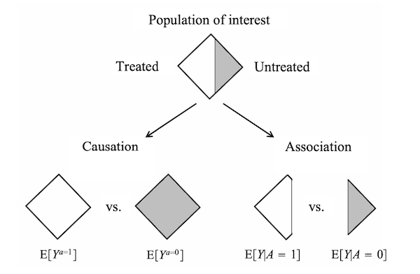
In essence, association is not causation. Causation is defined by a different risk in the same population under the two different treatment values, $P(Y^{a}=1)$, $a=1$ or $a=0$. That is, causal inference is concerned with what if, what would be the risk if everybody had been treated or untreated?

Association is defined by a different risk in two disjoint subsets of the population determined by the individual’s actual treatment value, $P(Y=1 \vert A=a)$, $A=1$ or $A=0$. Thus, associative inference is concerned with reality, what is the risk in the treated or the untreated?

In real word data, we can only observe the outcomes that indeed happened. The question is then under which conditions real world data can be used for causal inference. One approach is to conduct randomized experiments.

Randomized Experiments

Randomized experiments generate data with missing values of the counterfactual outcomes. However, randomization ensures that those missing values occurred by chance.

To make causal inference in randomized experiments, the assumption of exchangeability is required. When the group membership is randomized, which particular group received the treatment is irrelevant for the value of $P(Y=1 \vert A=1)$ and $P(Y=1 \vert A=0)$.

\[P(Y^{a}=1 \vert A=1) = P(Y^{a}=1 \vert A=0) = P(Y^{a}=1)\]

It means that the counterfactual risk under treatment value $a$ is the same in both groups $A=1$ and $A=0$. The treated and the untreated would have experienced the same risk of death if they had received the same treatment level (either $a=0$ or $a=1$). Thus, in ideal randomized experiments, association is causation.

\[\begin{aligned} P(Y^{a=1}=1) &= P(Y=1 \vert A=1) \\ P(Y^{a=0}=1) &= P(Y=1 \vert A=0) \end{aligned}\]

Formally, exchangeability is defined as independence between the counterfactual outcome and the actual treatment.

\[\ind{Y^{a}}{A}, \forall a\]

When the treated and the untreated are exchangeable, we say that treatment is exogenous. Exogeneity is commonly used as a synonym for exchangeability.

Note: $\ind{Y^{a}}{A}$ is different from $\ind{Y}{A}$. In a randomized experiment in which exchangeability $\ind{Y^{a}}{A}$ holds and the treatment has a causal effect on the outcome, then $\ind{Y}{A}$ does not hold because the treatment is associated with the observed outcome.

In practice, we are generally unable to determine whether exchangeability holds in our study. However, it is still possible that a study is a randomized experiment if exchangeability does not hold.

With some prognostic factor $L$ measured before treatment was assigned, we can conduct a study that is a randomized experiment with randomization conditional on $L$. We call it a conditionally randomized experiment.

Conditional randomization ensures that the treated and the untreated are exchangeable in the subset of individuals in the population, e.g., $L=1$ and $L=0$.

\[\begin{aligned} P(Y^{a}=1 \vert A=1, L=1) &= P(Y^{a}=1 \vert A=0, L=1) \\ P(Y^{a}=1 \vert A=1, L=0) &= P(Y^{a}=1 \vert A=0, L=0) \end{aligned}\]

Formally, conditional exchangeability is defined as independence between $Y^{a}$ and $A$ in different subsets of the population where $L=l$ for all $l$.

\[\cind{Y^{a}}{A}{L}, \forall a\]

In conditionally randomized experiments, we can compute the average causal effect in each of these subsets or strata of the population. Because association is causation within each subset, the stratum-specific causal risk ratio $\frac{P(Y^{a=1}=1 \vert L=1)}{P(Y^{a=0}=1 \vert L=1)}$ among people within $L=1$ is equal to the stratum-specific associational risk ratio $\frac{P(Y=1 \vert L=1, A=1)}{P(Y=1 \vert L=1, A=0)}$ among people within $L=1$. And analogously for $L=0$.

This method to compute stratum-specific causal effects is referred to as stratification. If the stratum-specific causal effects in each subset are different, we say that the treatment effect is modified by $L$, or that there is effect modification by $L$.

Standardization

There are two methods to compute the average causal effects in the whole population in a conditionally randomized experiment: standardization and inverse probability weighting.

Using standardization, the marginal counterfactual risk $P(Y^{a}=1)$ is the weighted average of the stratum-specific risks:

\[\begin{aligned} P(Y^{a}=1 ) &= \sum_{l}P(Y^{a}=1 \vert L=l) \cdot P(L=l) \\ &= \sum_{l}P(Y=1 \vert A=a, L=l) \cdot P(L=l) \end{aligned}\]

In the precense of conditional exchangeability, the standardized risk can be interpreted as the counterfactual risk that woud have been observed had all the individuals in the population been treated.

Inverse Probability Weighting

By weighting each individual in the population by the inverse of the conditional probability of receiving the treatment level that she indeed received, $W^{A}=1/f(A \vert L)$, we simulate a pseudo-population. Then, under conditional exchangeability in the original population, the treated and the untreated are (unconditionally) exchangeable in the pseudo-population because $L$ is independent of A.

Standardization and IP weighting are mathematically equivalent, both of which are based on the assumption that the variable $L$ had not been used to decide the probability of treatment.

Observational Studies

An observational study can be viewed as a conditionally randomized experiment if the following conditions hold:

1. Consistency: The values of treatment under comparison correspond to well-defined intervention that, in turn, correspond to the versions of treatment in the data.

2. Exchangeability: The conditional probability of receiving every value of treatment, though not decided by the investigators, depends only on the measured covariates $L$.

3. Positivity: The probability of receiving every value of treatment conditional on $L$ is greater than zero.

Note: An average causal effect is identifiable under a particular set of assumptions if these assumptions imply that the distribution of the observed data is compatible with a single value of the effect measure. It is unidentifiable if these assumptions imply that the distribution of the observed data is compatible with several values of the effect measure.

Exchangeability

In randomized experiments, the independent predictors of the outcome are equally distributed between the treated and the untreated.

\[\ind{Y^{a}}{A}, \forall a\]

In conditionally randomized experiments, within levels of $L$, all other predictors of the outcome are equally distributed between the treated and the untreated.

\[\cind{Y^{a}}{A}{L}, \forall a\]

If there exist unmeasured independent predictors $U$ of the outcome such that the probability of receiving teatment $A$ depends on $U$ within strata of $L$, then conditional exchangeability will not hold.

Positivity

There is positivity if $P(A=a \vert L=l) > 0, \forall a,l$. Positivity is only required for the variable $L$ that are required for exchangeability.

Consistency

Consistency is defined as the observed outcome for every treated individual equals her outcome if she had received treatment, that is $Y^{a}=Y$ for every individual with $A=a$. To ensure consistency, it needs sufficiently well-defined interventions $a$, in order to link the counterfactual outcomes $Y^{a}$ to the observed outcomes $Y^{A}=Y$, for individuals with $A=a$. It also needs positivity.